R语言临床预测模型讲义3:临床预测模型常见图表介绍
- 2026-04-12 02:57:16

一、预测模型变量探索和特征筛选
1. 基线表
注意事项:
描述统计形式:连续型:正态近似 → 均值±SD;偏态 → 中位数(IQR);分类/二分类:n(%) **明确单位:mmol/L、×10⁹/L 等; 表名: 在表格上方,简短表示,不要太复杂,简约易懂; 表注:在表格下方,包括:统计量: 连续型变量正态分布用均值±SD,非正态用中位数(IQR);分类变量用n(%);基线取值规则: 体征与实验室指标取“入院后2小时内首次记录”;SOFA为入院24小时内最高值;缺失处理: 表中缺失为插补前缺失率;模型训练采用多重插补(m=5);写清楚缩写例如: IQR,四分位距;SOFA,序贯器官衰竭评分;ACEI/ARB,血管紧张素转换酶抑制剂/受体阻滞剂。
作用和意义:
展示研究人群特征(描述样本) 比较分组间的平衡性或差异性 支撑模型变量选择与解释 增强模型研究的透明度与可比较性
2. 所有基线特征的ROC曲线和AUC (不是必要的)
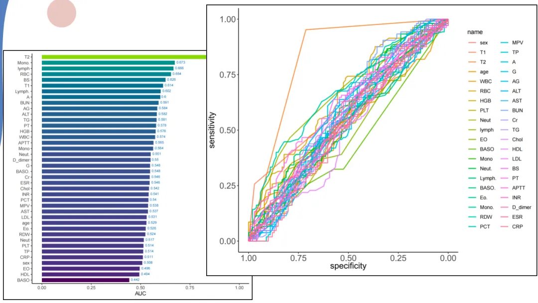
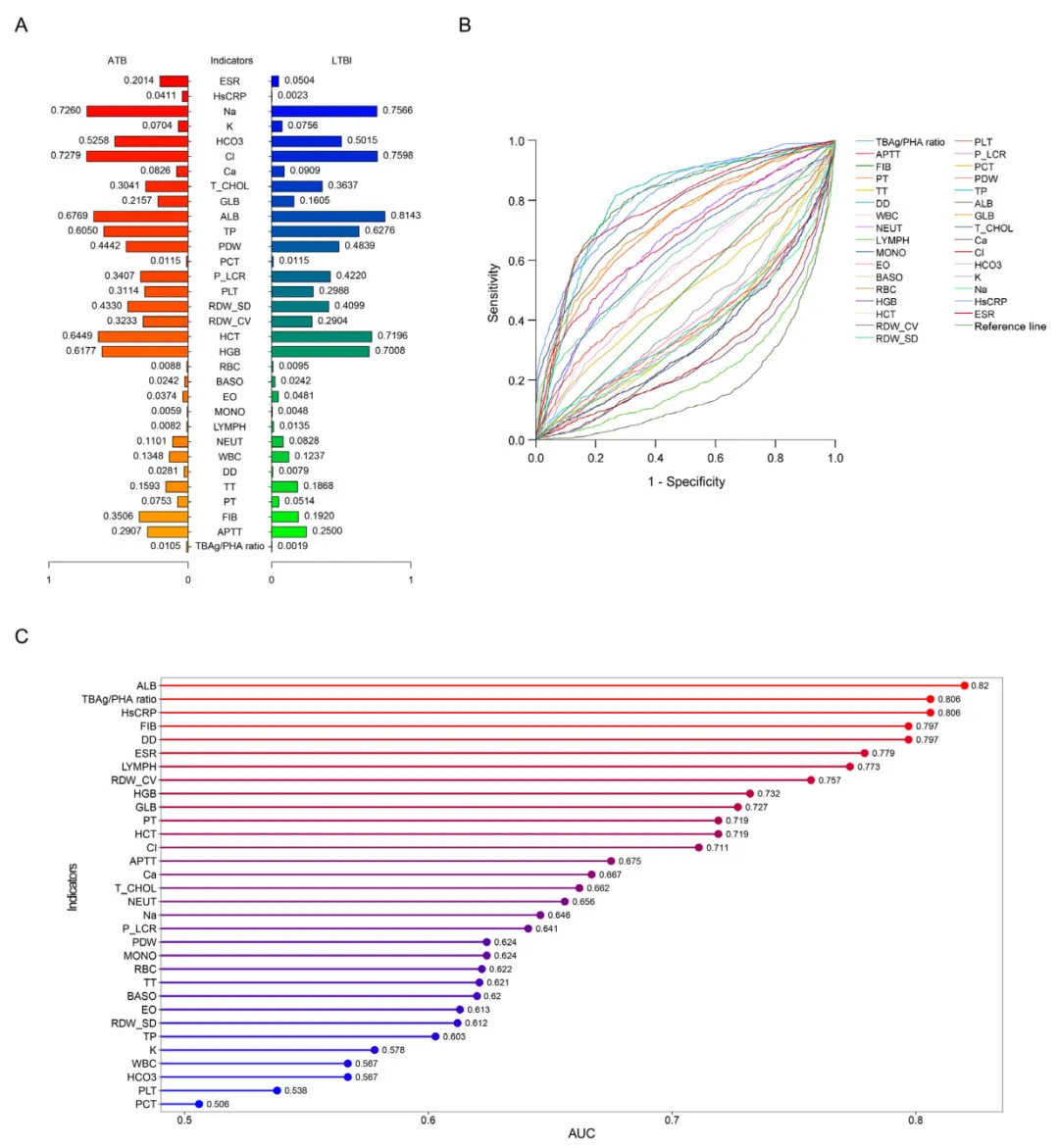
注意事项:
描述统计形式: ROC曲线用于评估每个变量(连续型或二分类变量)对结局事件的区分能力,采用AUC(Area Under Curve)作为定量指标。 图名: 图1. 各单变量ROC曲线与AUC柱状图
作用和意义:
评估单变量预测能力:通过AUC值,直观比较每个候选变量在区分“事件组与非事件组”上的性能,筛选出潜在的高价值预测因子。 指导多变量建模:AUC较高的变量(如>0.70)提示具有较强判别能力,可优先纳入后续多因素模型,但需结合临床意义与共线性评估。 揭示模型特征贡献差异:AUC柱状图可展示不同变量之间的区分度差异,有助于发现数据中主导信号与辅助特征。 验证数据一致性与合理性:若某些变量AUC接近0.5(无判别力),应反思该指标的测量稳定性或是否存在噪声干扰。 增强研究透明度:完整呈现单变量ROC结果,可帮助审稿人判断模型输入变量的合理性与独立信息量,提升研究的可解释性。
3. 相关性热图
相关系数 r [-1,1], p(样本量小的时候用)
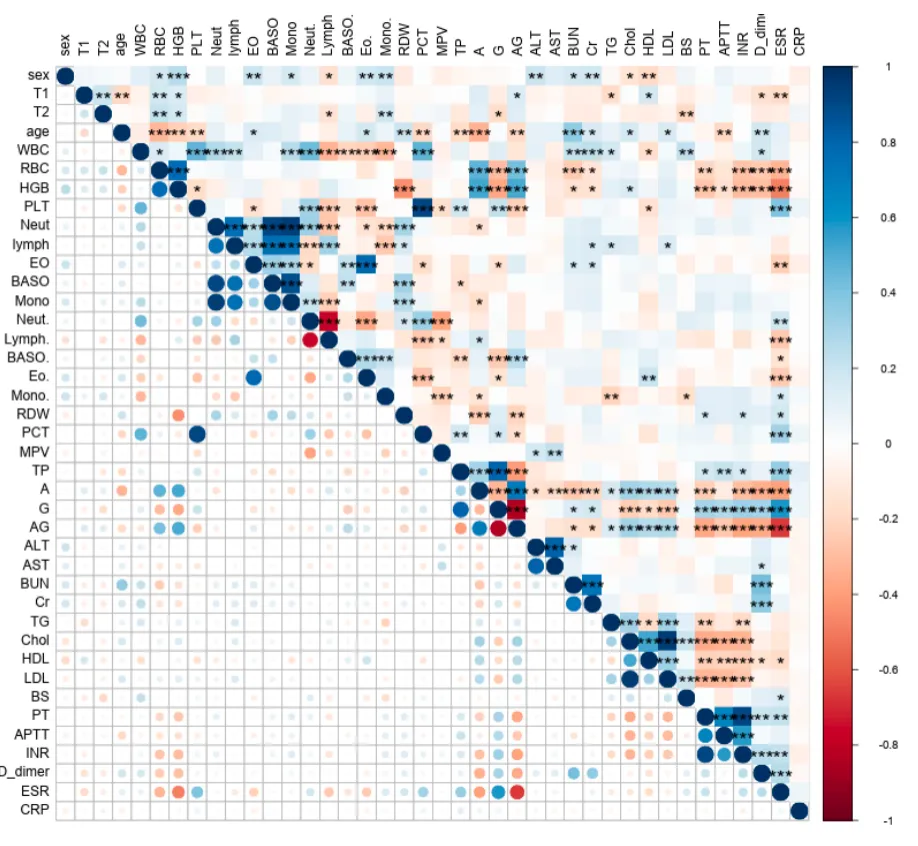
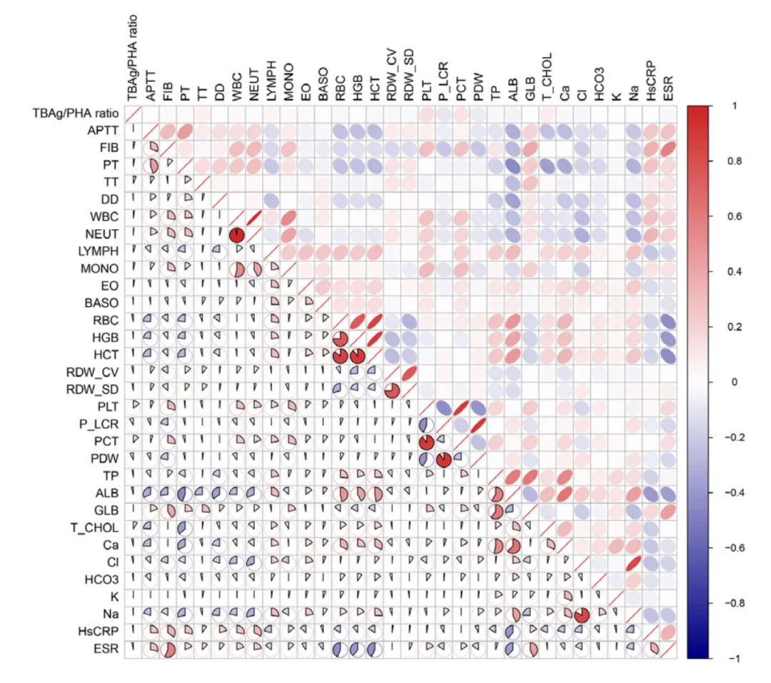
注意事项:
数据来源: 纳入模型前的所有候选变量,分类变量经哑变量编码; 计算方法: 采用Spearman或Pearson相关系数,根据变量分布特征选择; 显著性表示: p<0.05以星号标注或通过颜色深浅体现; 图名: 图2. 所有候选变量间的相关性热图 图注: 统计量说明: 热图中颜色代表相关系数r的大小,范围[-1,1],正相关为红色,负相关为蓝色; 缩写示例: HR,心率;SBP,收缩压;DBP,舒张压;WBC,白细胞计数;CRP,C反应蛋白;ALT,丙氨酸转氨酶。
作用与意义:
揭示变量间依赖结构: 通过热图可直观识别高度相关的变量对,为后续变量筛选与共线性处理提供依据。 指导特征选择与建模: 当两变量相关性极高(|r|>0.8),可考虑在建模时仅保留其中一个,以减少冗余信息与模型不稳定性。 发现潜在生物学/临床联系: 变量间的强相关可能反映共同的病理生理过程(如炎症指标聚集)。 验证数据一致性: 若出现反常相关(如两个理论无关变量高相关),提示可能存在编码或数据录入错误。 提升可解释性与模型透明度: 热图作为模型建立前的全局探索性可视化,帮助读者理解变量结构、模型复杂度与数据质量。
4. Lasso回归(变量筛选)
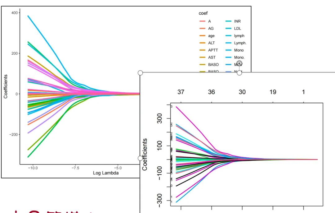
LASSO回归系数路径图(LASSO coefficient path plot):
数据说明: 横轴为正则化参数 λ(取对数后展示),纵轴为各变量的回归系数。 绘图含义: 每条曲线代表一个变量的系数随λ变化的路径,当λ增大时,系数逐渐趋近于0。 模型设置: 使用10折交叉验证(cv.glmnet),标准化所有连续变量,分类变量经哑变量编码。 图名: 图3. LASSO回归路径图(Coefficient profile plot) 图注: 统计量说明: λ越大,惩罚项越强,模型越稀疏;当λ趋大时,大部分变量系数被压缩为0,仅保留最具预测力的特征。 变量选择: 图中可视化展示了特征逐步被剔除的过程,有助于观察模型稀疏化趋势。 缩写示例: LASSO,最小绝对收缩与选择算子(Least Absolute Shrinkage and Selection Operator);λ,惩罚系数。
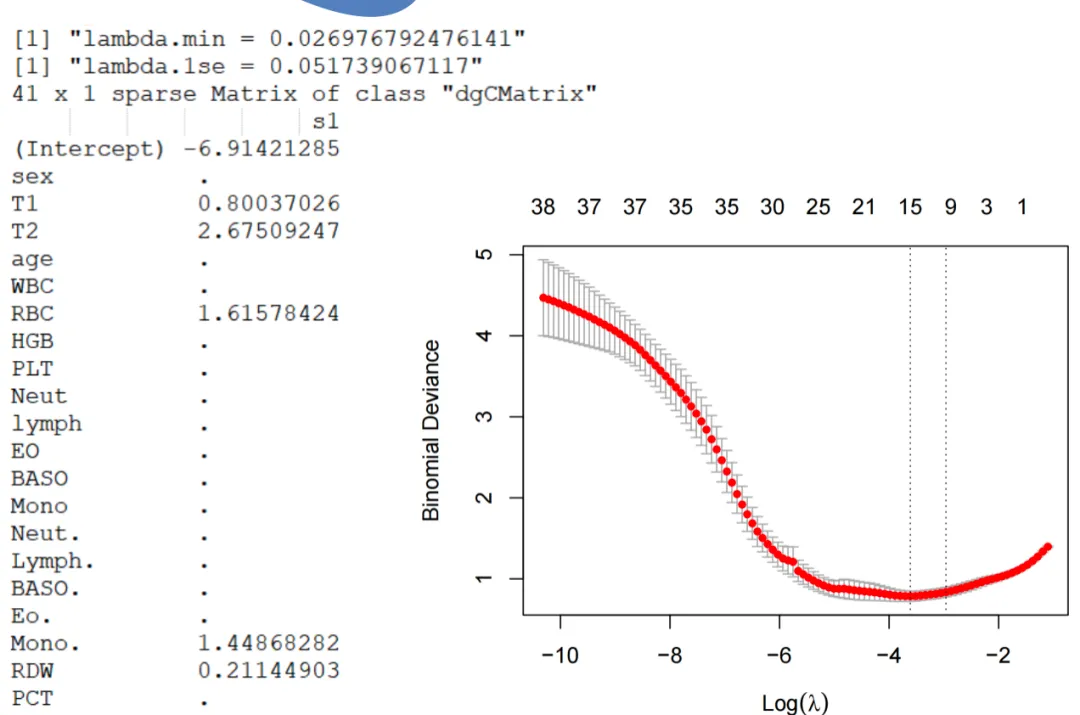
LASSO交叉验证曲线图(Cross-validation curve):
数据说明: 横轴为正则化参数 λ(取对数后展示),纵轴为交叉验证误差(如偏差或均方误差)。 绘图含义: 实线为平均误差,误差条为±1标准误差范围;两条垂线分别对应λ_min(误差最小)和λ_1se(误差在1标准误差内的最简模型)。 图名: 图4. LASSO模型的10折交叉验证结果(Cross-validation curve for λ selection) 图注: 统计量说明: 通过最小化交叉验证误差确定最优惩罚系数λ;λ_min用于最佳拟合,λ_1se用于更简约、泛化性更好的模型。 模型选择标准: 通常选取λ_1se作为最终模型,以平衡模型性能与简约性。 缩写示例: MSE,均方误差;SE,标准误差;λ_min,最小误差对应λ;λ_1se,1标准误差范围内最简λ。
Data driven variable selection methods [https://pmc.ncbi.nlm.nih.gov/articles/PMC11369751/#sec22]数据驱动的变量选择方法We advise against univariable selection methods—that is, methods that test each predictor separately and retain only statistically significant predictors. These methods do not consider the association between predictors and could lead to loss of valuable information.55[https://pmc.ncbi.nlm.nih.gov/articles/PMC11369751/#ref55] 66[https://pmc.ncbi.nlm.nih.gov/articles/PMC11369751/#ref66] Stepwise methods for variable selection (eg, forward, backwards, or bidirectional variable selection) are commonly used. Again, they are not recommended because they might lead to bias in estimation and worse predictive performance.55[https://pmc.ncbi.nlm.nih.gov/articles/PMC11369751/#ref55] 67[https://pmc.ncbi.nlm.nih.gov/articles/PMC11369751/#ref67] 68[https://pmc.ncbi.nlm.nih.gov/articles/PMC11369751/#ref68] If variable selection is desirable—for instance, to simplify the implementation of the model by further reducing the number of predetermined predictors—more suitable methods can be used as described below.我们不建议使用单变量选择方法——即那些对每个预测变量分别检验并仅保留统计学上显著的预测变量的方法。这些方法没有考虑预测变量之间的关联,可能导致有价值信息的丢失。向前、向后或双向变量选择等逐步方法在变量选择中常被使用。但同样不推荐这些方法,因为它们可能导致估计偏倚和更差的预测性能。 如果需要进行变量选择——例如,为了进一步减少预先确定的预测变量数量以简化模型的实施——可以使用下面所述的更合适的方法。Model estimation 模型估计Adding penalty terms to the model (a procedure called penalisation, regularisation, or shrinkage; see table 1[https://pmc.ncbi.nlm.nih.gov/articles/PMC11369751/#tbl1]) is recommended to control the complexity of the model and prevent overfitting.69[https://pmc.ncbi.nlm.nih.gov/articles/PMC11369751/#ref69] 70[https://pmc.ncbi.nlm.nih.gov/articles/PMC11369751/#ref70] 71[https://pmc.ncbi.nlm.nih.gov/articles/PMC11369751/#ref71] Penalisation methods such as ridge, LASSO (least absolute shrinkage and selection operator), and elastic net generally lead to smaller absolute values of the coefficients—that is, they shrink coefficients towards zero—compared with maximum likelihood estimation.72[https://pmc.ncbi.nlm.nih.gov/articles/PMC11369751/#ref72] LASSO and elastic net can be used for variable selection (similar to the methods described above). These models might exclude some predictors by setting their coefficients to zero, leading to a more interpretable and simpler model. Machine learning methods typically also have penalisation embedded. Penalisation is closely related to the bias-variance trade-off depicted in figure 1[https://pmc.ncbi.nlm.nih.gov/articles/PMC11369751/#f1], and is a method aiming to bring the model closer to the sweet spot of the bias-variance trade-off curve, where model performance in new data is maximised (note that the figure does not include a description of the double descent phenomenon).73[https://pmc.ncbi.nlm.nih.gov/articles/PMC11369751/#ref73] Although penalisation methods have advantages, they do not solve all the problems associated with small sample sizes. While these methods typically are superior to standard estimation techniques, they can be unstable in small datasets. Moreover, their application does not ensure improved predictive performance.74[https://pmc.ncbi.nlm.nih.gov/articles/PMC11369751/#ref74] 75[https://pmc.ncbi.nlm.nih.gov/articles/PMC11369751/#ref75]向模型添加惩罚项(称为惩罚、正则化或收缩;见表 1)被建议用于控制模型复杂性并防止过拟合。 与极大似然估计相比,诸如岭回归、LASSO(最小绝对收缩与选择算子)和弹性网等惩罚方法通常会使系数的绝对值更小——即将系数收缩到零附近。 LASSO 和弹性网可用于变量选择(类似于上述描述的方法)。这些模型可能通过将某些预测变量的系数设为零来将其排除,从而得到更易解释且更简单的模型。机器学习方法通常也内嵌有惩罚机制。惩罚与图 1 所示的偏差-方差权衡密切相关,是一种旨在将模型拉近偏差-方差权衡曲线甜蜜点的方法,以在新数据上最大化模型性能(注意该图未包含双重下降现象的描述)。虽然惩罚方法具有优点,但它们并不能解决与样本量小相关的所有问题。尽管这些方法通常优于标准估计技术,但在小型数据集中可能不稳定。此外,应用这些方法并不保证能提升预测性能。
二、二分类预测模型常见图表
1. 多因素回归表格(Logistic回归)和森林图
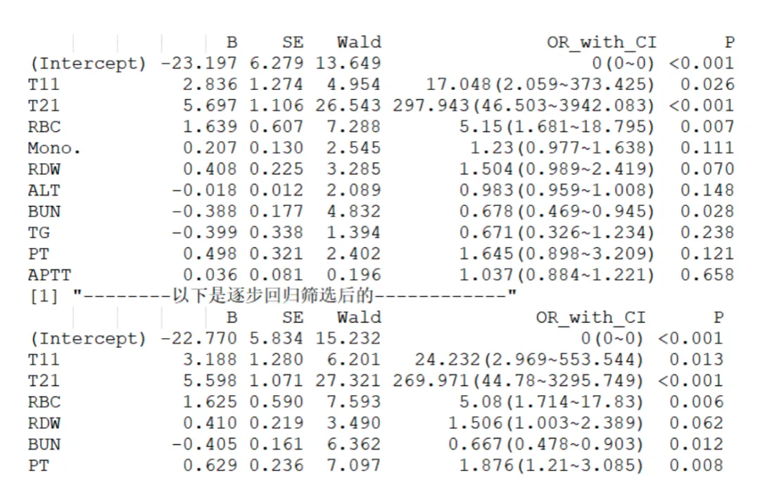
多因素回归表格中显著性的问题:在模型解释中,单个变量的统计显著性(P值)并不是决定其是否保留的唯一标准。对于预测模型而言,更重要的是变量整体的预测能力与模型稳定性。一个变量即使P值略高,也可能提升模型的拟合度、改善判别能力(如AUC)或增强模型的临床可解释性。因此,我们不应机械地以P<0.05为筛选依据。但是这个是可以主观选择的,你也可以为了平衡模型复杂度与稳健性,进一步采用逐步回归(stepwise selection) 方法,在AIC(Akaike信息准则)或BIC(贝叶斯信息准则)标准下自动筛选变量,剔除对模型贡献有限的冗余因素,从而获得更简约的最终模型。该策略既避免过度拟合,又保持模型在临床应用中的简洁与可操作性。
结果解读
| (Intercept) | ||||
| T1 = 1 | ||||
| T2 = 1 | ||||
| RBC | ||||
| RDW | ||||
| BUN | ||||
| PT | ||||
| 整体解读: | ||||
| RDW(P=0.062)虽未达到传统显著水平,但仍呈现出潜在趋势性 |
系数(B值)方向解释:
B>0 表示变量升高(或事件存在)增加结局发生概率; B<0 表示变量升高减少结局发生概率。 例如,BUN为负值,提示其升高具有保护作用。 OR值的解读范围: OR>1 表示变量升高或者事件存在增加结局发生的概率; OR<1 表示变量升高或者事件发生减少发生概率
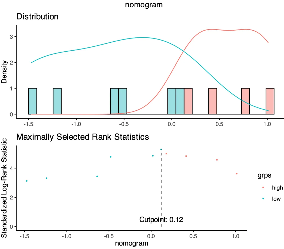
2. 列线图(Nomogram)
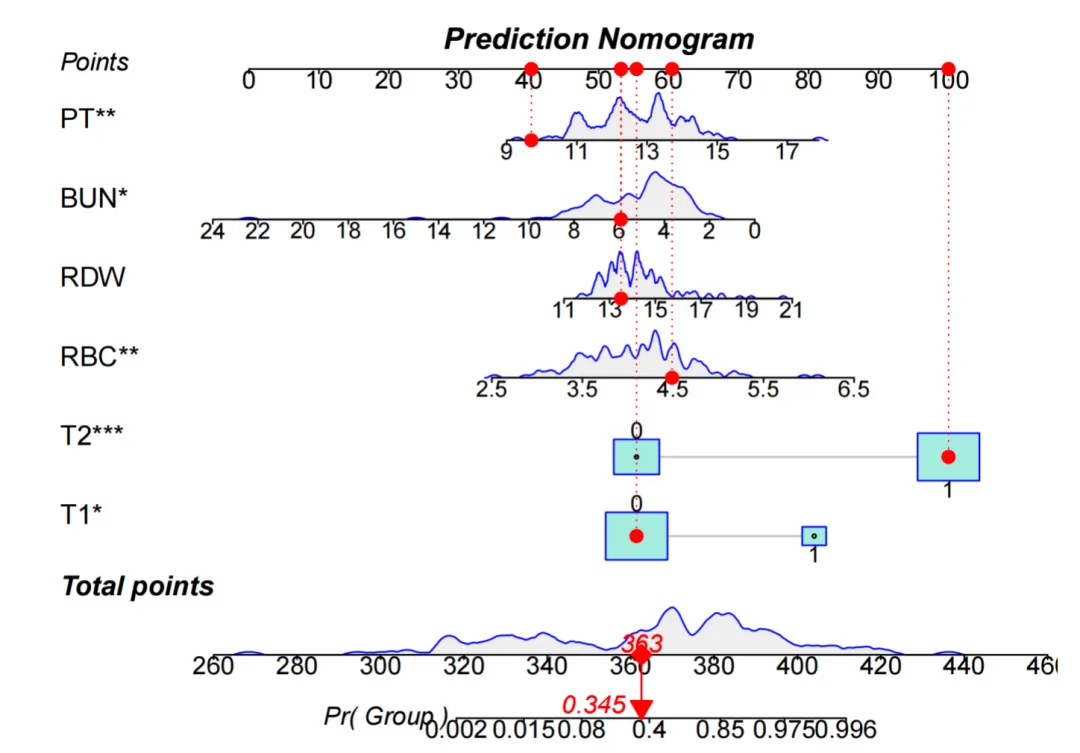
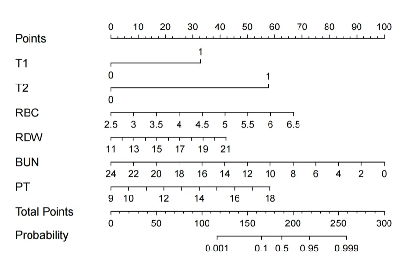
回答的问题:如何把回归模型直观地用于临床沟通与手工估算? 何时使用:需要快速估算风险。 怎么读:变量打点 → 总分 → 风险。 1 句话解释示例: “患者 A 总分 165,对应xxx风险约 18%,建议进入进一步评估通道。”
模型预测结果的三种形式
在临床预测模型中,我们通常会得到三种不同但密切相关的结果:
真实标签(True Label) 这是每位患者在研究中的实际结局,例如是否死亡、是否治疗失败等。 一般用 0表示未发生事件,1表示发生事件。这是模型学习的“目标变量”,用来训练和验证模型。 预测概率(Predicted Probability) 这是模型输出的连续值,表示每位患者发生事件的风险概率。 例如 Logistic 回归模型输出 0.0–1.0 之间的值。 值越高,模型认为患者越有可能发生事件。 示例:患者A=0.85、患者B=0.30、患者C=0.10。 预测标签(Predicted Label) 当我们设定一个截断值(cut-off)(例如0.5),可以将连续概率转化为二分类结果: 若预测概率 ≥ 0.5 → 预测为“事件发生”(1) 若预测概率 < 0.5 → 预测为“事件未发生”(0) 截断值的选择会影响模型的灵敏度与特异度,可通过 ROC 曲线或 Youden 指数确定最优 cut-off。
在做完模型后我们可以通过predict等类似函数得到模型在不同数据集的每一个患者的预测概率
3. 模型的ROC 曲线(Receiver Operating Characteristic)
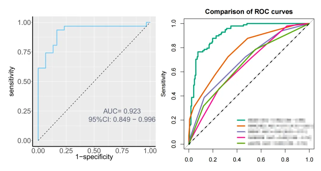
ROC曲线(Receiver Operating Characteristic curve)用于评估模型区分事件组与非事件组的能力;AUC(曲线下面积)反映模型总体判别性能。
数值范围: AUC = 0.5 表示无判别力(等同随机); 0.7 ≤ AUC < 0.8 表示可接受; 0.8 ≤ AUC < 0.9 表示良好; AUC ≥ 0.9 表示极佳。 绘图说明: ROC曲线横轴为1–特异度(1–Specificity),纵轴为敏感度(Sensitivity); 虚线代表随机分类线(AUC=0.5); 常见误区:不平衡数据(低发生率/高发生率结局)只看 AUC 容易“看着好”,请同时查看 PR 曲线。
4. 模型的内部验证
BMJ临床预测模型指南[https://pmc.ncbi.nlm.nih.gov/articles/PMC11369751/#sec22]The simplest method is the split sample approach where the dataset is randomly split into two parts (eg, 70% training and 30% testing). However, this method is problematic because it wastes data and decreases statistical power.55[https://pmc.ncbi.nlm.nih.gov/articles/PMC11369751/#ref55] 87[https://pmc.ncbi.nlm.nih.gov/articles/PMC11369751/#ref87] When applied to a small dataset, it might create two datasets that are inadequate for both model development and evaluation. Conversely, for large datasets it offers little benefit because the risk of overfitting is low. Further, it might encourage researchers to repeat the procedure until they obtain satisfactory results.88[https://pmc.ncbi.nlm.nih.gov/articles/PMC11369751/#ref88] Another approach is to split the data according to the calendar time of patient enrolment. For example, we might develop the model using data from an earlier period and test it in patients enrolled later. This procedure (temporal validation)35[https://pmc.ncbi.nlm.nih.gov/articles/PMC11369751/#ref35] 89[https://pmc.ncbi.nlm.nih.gov/articles/PMC11369751/#ref89] might inform us about possible time trends in model performance. However, the time point used for splitting the data will generally be arbitrary and older data might not reflect current patient characteristics or health care. Therefore, this approach is not recommended for the development phase.88[https://pmc.ncbi.nlm.nih.gov/articles/PMC11369751/#ref88]最简单的方法是样本分割法,即随机将数据集分为两部分(例如 70%训练集和 30%测试集)。但这种方法存在缺陷,会造成数据浪费并降低统计效能。当应用于小规模数据集时,可能产生两个既不足以开发模型也不足以评估模型的子集。反之,对于大规模数据集则益处不大,因为过拟合风险本身较低。此外,这种方法可能促使研究者重复操作直至获得满意结果。另一种方法是根据患者入组时间进行数据分割。例如使用早期数据开发模型,在后入组患者中测试。这种时序验证方法可以揭示模型性能可能存在的时间趋势。但数据分割时点通常具有主观性,且早期数据可能无法反映当前患者特征或医疗状况。因此不建议在开发阶段采用这种方法。A better method is k-fold cross validation. In this approach, we divide the data randomly in k (usually 10) subsets (folds). The model is built using k−1 of these folds and evaluated on the remaining one fold. This process is repeated, cycling through all the folds so that each can be the testing set. The model's performance is measured in each cycle, and the k estimates are then combined and summarised to get a final performance measure. Bootstrapping is another method,90[https://pmc.ncbi.nlm.nih.gov/articles/PMC11369751/#ref90] which can be used to calculate optimism and optimism corrected performance measures for any model. Box 2[https://pmc.ncbi.nlm.nih.gov/articles/PMC11369751/#box2] outlines the procedure.47[https://pmc.ncbi.nlm.nih.gov/articles/PMC11369751/#ref47] Bootstrapping generally leads to more stable and less biased results,93[https://pmc.ncbi.nlm.nih.gov/articles/PMC11369751/#ref93] and is therefore recommended for internal validation.47[https://pmc.ncbi.nlm.nih.gov/articles/PMC11369751/#ref47] However, implementation of k-fold cross validation and bootstrapping can be computationally demanding when multiple imputation of missing data is needed.88[https://pmc.ncbi.nlm.nih.gov/articles/PMC11369751/#ref88]一种更优的方法是 k 折交叉验证[https://www.bilibili.com/video/BV1GQ4y1P7Tv/?spm_id_from=333.337.search-card.all.click&vd_source=265a67059f8104931870be807f794a7f]。该方法将数据随机划分为 k 个(通常为 10 个)子集(折)。模型使用其中 k-1 折数据构建,并在剩余的 1 折数据上进行评估。此过程循环重复,使每个子集都能作为测试集。每次循环都测量模型性能,最终汇总 k 次评估结果得出综合性能指标。自助法(Bootstrap)是另一种方法 90 ,可用于计算任何模型的乐观偏差及经乐观修正后的性能指标,具体步骤见方框 2 47 。自助法通常能获得更稳定、偏差更小的结果 93 ,因此推荐用于内部验证 47 。但需要注意的是,当需要进行多重缺失值填补时,k 折交叉验证和自助法的实施可能会产生较高的计算负荷 88 。
C指数 ≈ AUC
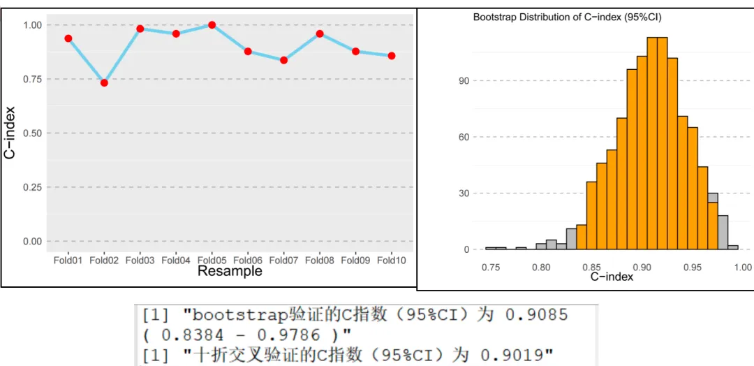
一、十折交叉验证的意义与优势
更稳定的评估: 十折交叉验证将数据划分为10个子集,轮流作为验证集,循环10次取平均性能。 → 减少单次划分带来的随机偏差,使模型评估更加稳定可靠。 充分利用数据: 每个样本都既参与训练又参与验证,在小样本临床研究中可最大化数据使用率。 结果解读(折线图): 蓝色折线:C指数在10次验证中的变化趋势。 红点:每次验证的具体C指数。 折线平稳、点分布集中 → 模型稳定;波动大 → 模型可能过拟合或数据异质性高。
二、Bootstrap自助法验证的意义与优势
模拟抽样分布: 通过有放回抽样构建多个自助样本(与原始样本量相同),评估模型在不同抽样下的稳健性。 → 能捕捉复杂数据结构对模型的影响,减少过拟合风险。 适用于小样本与复杂模型: 当样本有限或变量较多时,Bootstrap能提供更稳定的性能估计。 结果解读(直方图): 看分布形态:接近正态分布 → 模型稳健;偏态或多峰 → 模型不稳定。 看置信区间:区间窄 → 性能稳定;区间宽 → 需优化模型或检查数据。
三、与单次划分法相比的优势
减少评估偏差: 多次抽样或划分可全面反映模型表现,避免因一次划分造成的高估或低估。 更准确的泛化评估: 能更好地模拟模型在未见样本(新患者)上的表现,是临床预测模型可靠性的重要体现。
四、综合判断与模型解释
比较十折交叉验证的平均C指数与Bootstrap平均C指数,若两者接近,说明模型稳健、评估结果可信。 结合C指数数值与置信区间宽度判断模型性能: C指数高、置信区间窄 → 模型性能优良; C指数低或置信区间宽 → 可能需调整变量或简化模型。
5. 校准曲线(Calibration)
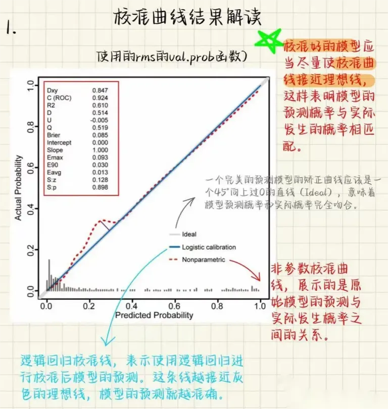
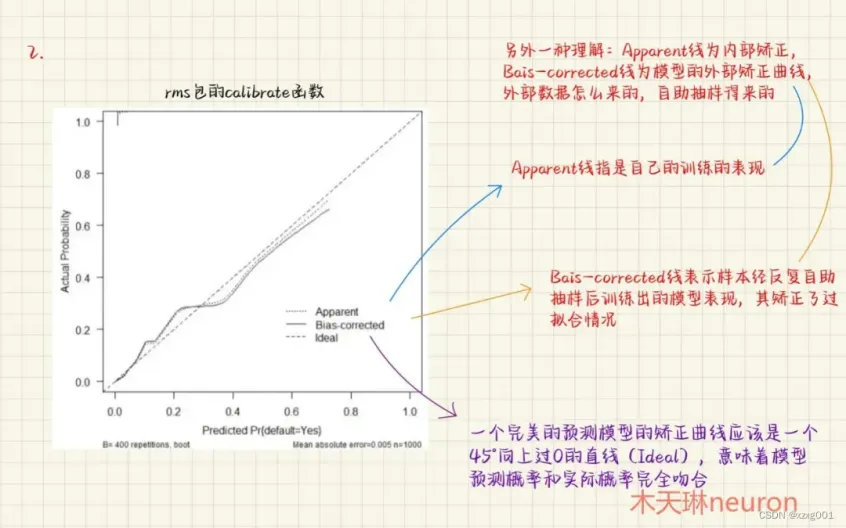
回答的问题:模型给出的概率本身准不准? 何时使用:所有预测“风险/概率”的模型都应报告。在进行Logistic回归临床预测模型的校准验证(Calibration)时,除了绘制校准曲线外,通常还会返回一系列统计指标,用于量化模型预测值与实际观测值的一致性。这些指标从不同角度评价模型的区分能力、拟合优度与可靠性 。两个图都是用的rms包进行绘制,左边的图会有一些详细的参数信息输出,以左图为例:
| Dxy = 0.847 | |
| C (ROC) = 0.924 | |
| R² = 0.610 | |
| D = 0.514 | |
| U = -0.005 | |
| Q = 0.519 | |
| Brier = 0.085 | |
| Intercept = 0.000 | |
| Slope = 1.000 | |
| Emax = 0.093 | |
| E90 = 0.030 | |
| Eavg = 0.013 | |
| S:z = 0.128, S:p = 0.898 |
6. 决策曲线分析(DCA, Decision Curve Analysis)
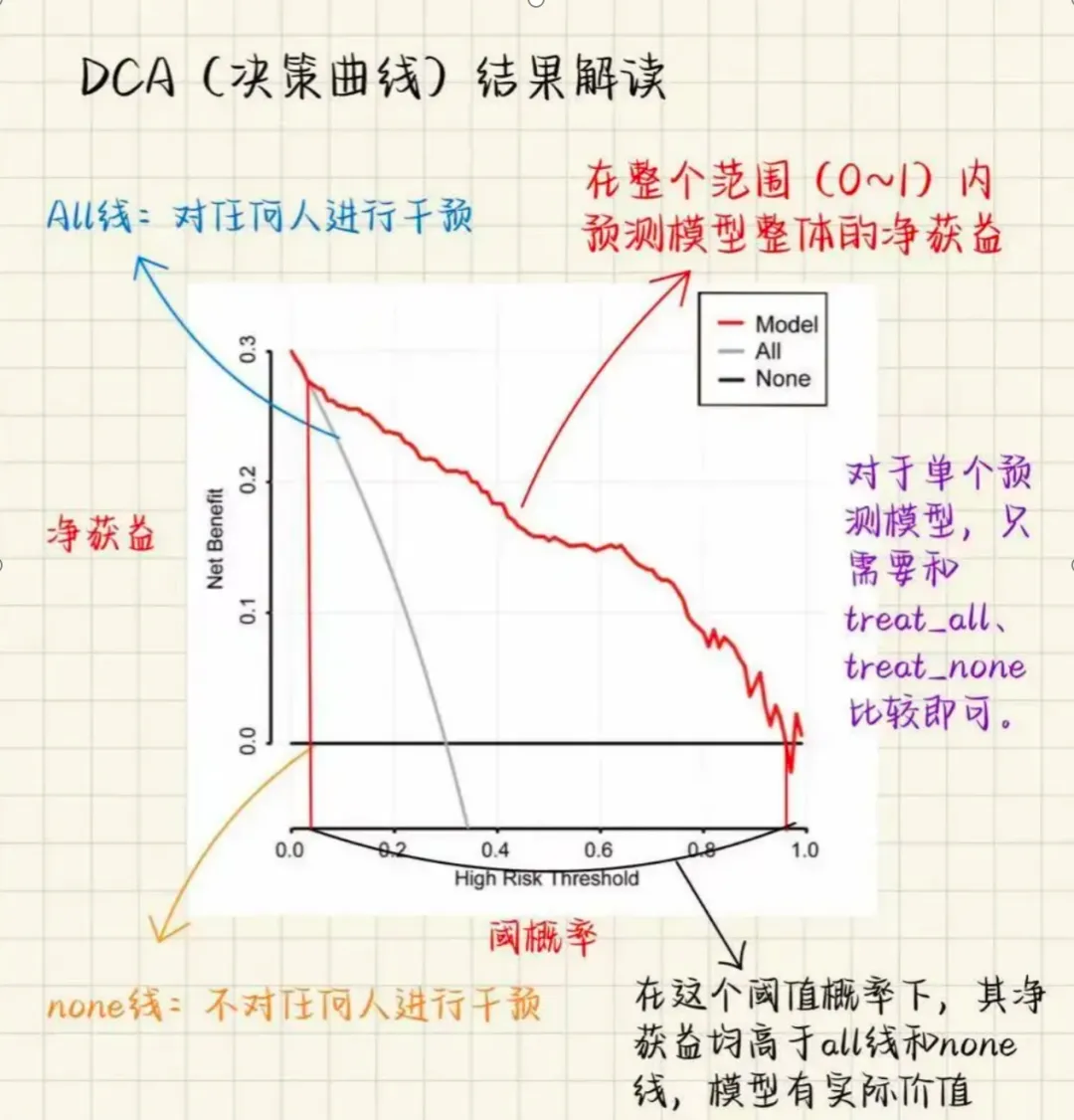
DCA曲线组成部分1)阈值概率:临床决策者采取某项干预措施的概率阈值。换言之,它是疾病的预测概率,超过该概率时,预期的治疗益处超过其带来的风险。2)净收益(Net Benefit):这是模型在特定阈值概率下的效用度量,考虑了真阳性带来的益处减去假阳性带来的损害(经适当加权)。3)净收益曲线(Net Benefit Curve)展示了在不同阈值概率下模型的净收益。通过比较不同模型的净收益曲线,可以直观地看出哪个模型在特定条件下更优。4)参考线(Reference Lines)在DCA图中,通常会包括几条参考线作为比较的基准,最常见的有:“不采取任何行动”(Treat None)的净收益线:假设没有患者被治疗,此时的净收益是零。“治疗所有患者”(Treat All)的净收益线:假设所有患者都接受治疗,这条线展示了在这种极端情况下的净收益。5)决策阈值(Decision Threshold)这是决策者做出治疗决策时考虑的阈值概率的具体值。在实际应用中,这个阈值是基于疾病的严重性、治疗的潜在风险与益处以及患者偏好等因素综合确定的。
7. 混淆矩阵热图(Confusion Matrix /指定阈值(根据ROC曲线确定的最佳截断值))
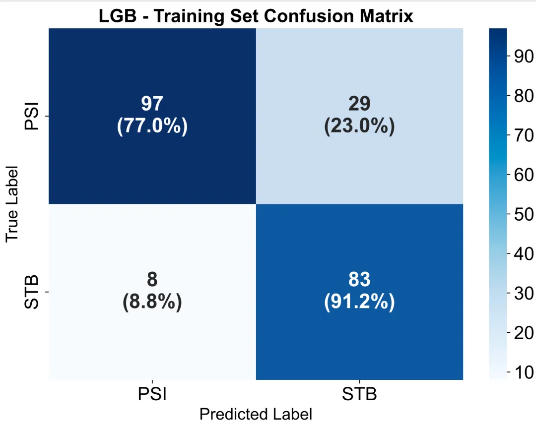
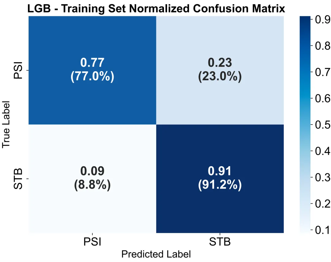
通过二维表格形式显示预测值与真实值的对应关系:对角线上的数值代表模型预测正确的样本数(真阳性与真阴性),非对角线表示预测错误的样本(假阳性与假阴性)。热图颜色深浅反映分类数量大小,颜色越深说明该类别预测越集中。通过观察混淆矩阵,可以判断模型在不同类别上的识别能力与误差类型,例如是否存在某一类被系统性误判。相比单一AUC指标,混淆矩阵能更直观地揭示模型在指定阈值下的分类性能平衡性(灵敏度、特异度、准确率)
基于混淆矩阵计算模型性能指标(Model Performance Metrics)
在二分类模型(如Logistic回归)中,我们常用以下统计指标来衡量模型在不同阈值下的预测表现。它们均来源于混淆矩阵:
| 阳性(Positive) | ||
| 阴性(Negative) | ||
1. 灵敏度(Sensitivity / Recall / True Positive Rate)
定义:模型正确识别出真实阳性病例的能力。公式:
理解:灵敏度越高,模型漏诊的可能性越低,临床上更关注于“不要漏掉真正的阳性”。
2. 特异度(Specificity / True Negative Rate)
定义:模型正确识别出真实阴性病例的能力。公式:
理解:特异度高说明模型“不会误报”,即假阳性率低。
3. 阳性预测值(PPV, Positive Predictive Value)
定义:预测为阳性的样本中,实际为阳性的比例。公式:
理解:反映模型阳性预测结果的“可信度”,受疾病患病率影响。
4. 阴性预测值(NPV, Negative Predictive Value)
定义:预测为阴性的样本中,实际为阴性的比例。公式:
理解:反映阴性预测的可靠性,NPV高说明阴性结果可信。
5. 准确率(Accuracy)
定义:模型所有预测中正确预测(包括阳性和阴性)的比例。公式:
理解:衡量总体预测正确率,但在样本不平衡(阳性/阴性比例悬殊)时不可靠。
6. F1分数(F1 Score)
定义:灵敏度(Recall)与阳性预测值(Precision)的调和平均。公式:
或
理解:在类别不平衡时,比准确率更能反映模型在正例上的综合表现。
三、生存结局常见图表
1. 时间依赖 ROC(AUC)/ C 指数
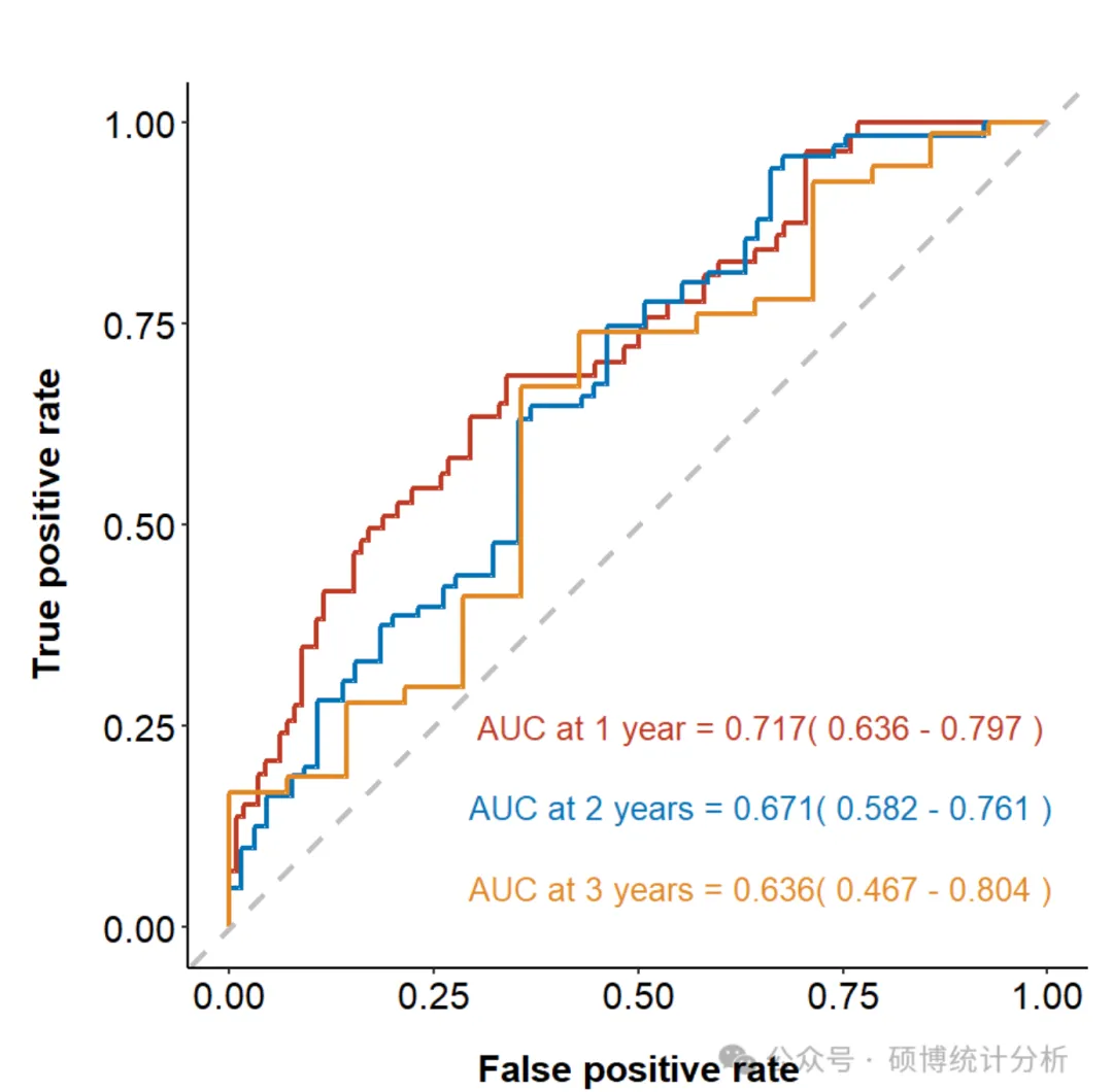
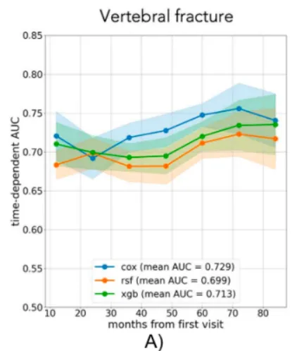
回答的问题:在不同随访时间点,模型区分“更早发生事件”的能力如何? 怎么读:报告 1/3/5 年 AUC(t) 或整体 C 指数; 1 句话解释示例: “1/3/5 年 AUC(t) 分别为 0.78/0.76/0.74;C指数为0.75。”
2. 固定时间点校准曲线(如 1/3/5 年)
回答的问题:在某个时间点,预测生存/事件概率是否校准良好? 1 句话解释示例: “3 年校准接近理想线。”
3. KM 风险分层曲线(Kaplan–Meier by Risk Groups)[[https://zhuanlan.zhihu.com/p/113676828]]
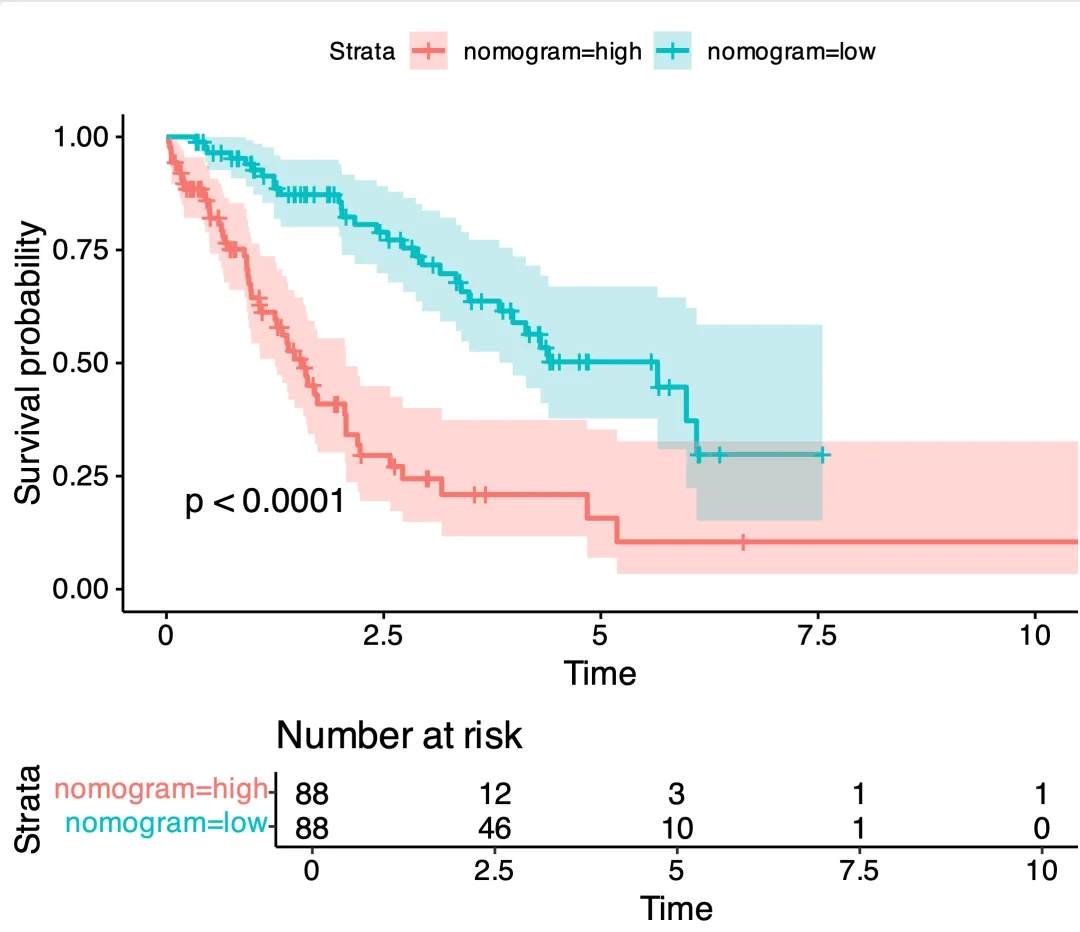
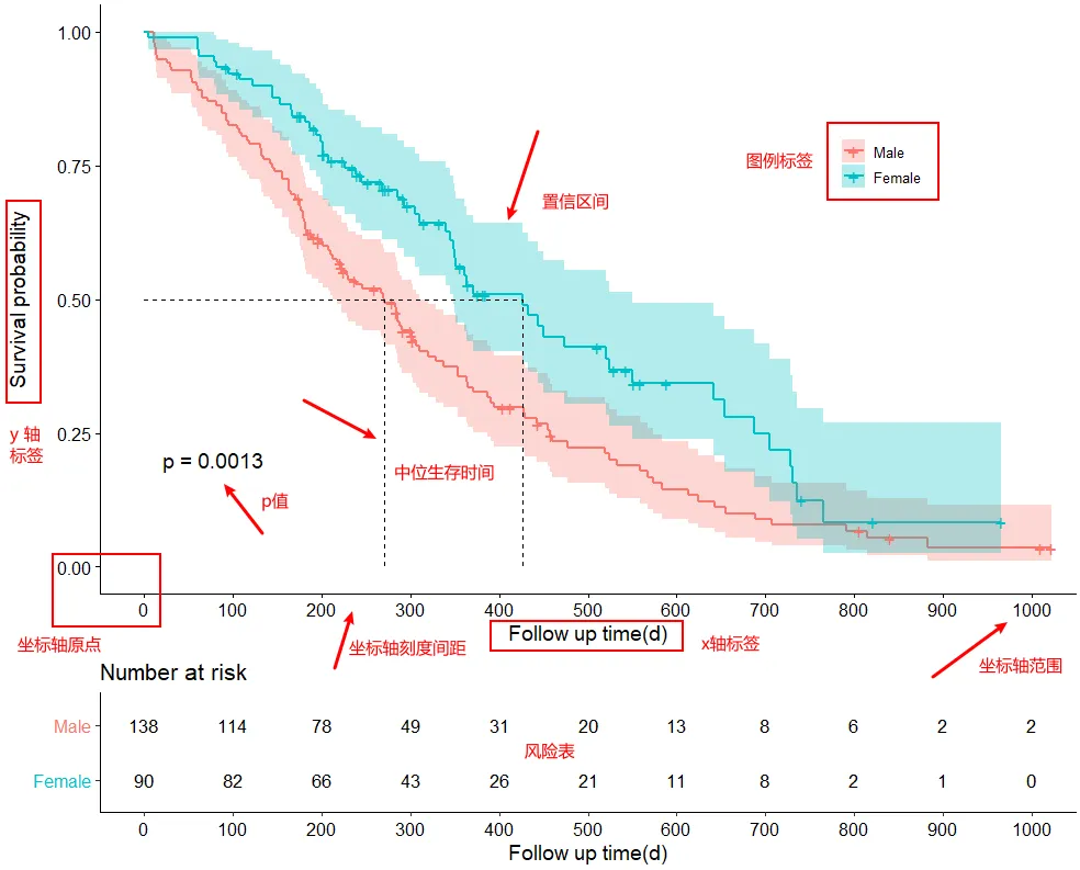
回答的问题:按预先定义的风险分组,生存曲线是否有显著差异?
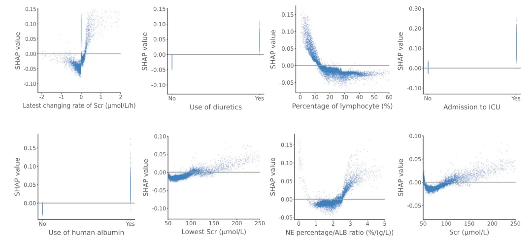
四、可解释机器学习模型SHAP可视化全解析

首先先把这个概念讲清楚:列线图(Nomogram)本质上是“线性可加”的可视化工具,它把模型的“线性预测器”(各变量系数加权求和)转成一个可读的打分尺,适合解释线性回归 / Logistic 回归 / Cox 回归这类具有明确系数、可加结构的模型。也正因为它依赖“系数 + 线性相加”,所以它并不是为随机森林、XGBoost、神经网络这类机器学习模型设计的解释方式。
但这并不意味着机器学习模型不能解释。恰恰相反:机器学习模型之所以需要更“专业”的解释框架,是因为它们往往是非线性、强交互、不可直接写出一个简单加和公式的模型。这个时候,我们就需要引入一套更通用的解释方法——SHAP(SHapley Additive exPlanations)。
1. 为什么机器学习模型不能直接画列线图?
对临床同学来说,可以用一句话理解:列线图依赖“系数”,而多数机器学习模型没有一组固定可解释的系数。
在 Logistic 回归里:每个变量都有一个系数 β,风险可以写成一个公式,变量贡献“相对稳定”。 在 XGBoost 里:模型由成百上千棵树组成,变量的影响会随着分裂路径变化,同一个变量在不同人身上可能贡献完全不同,还常常存在交互效应。 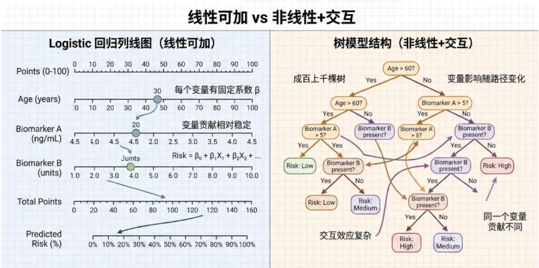
2. SHAP 在做什么?
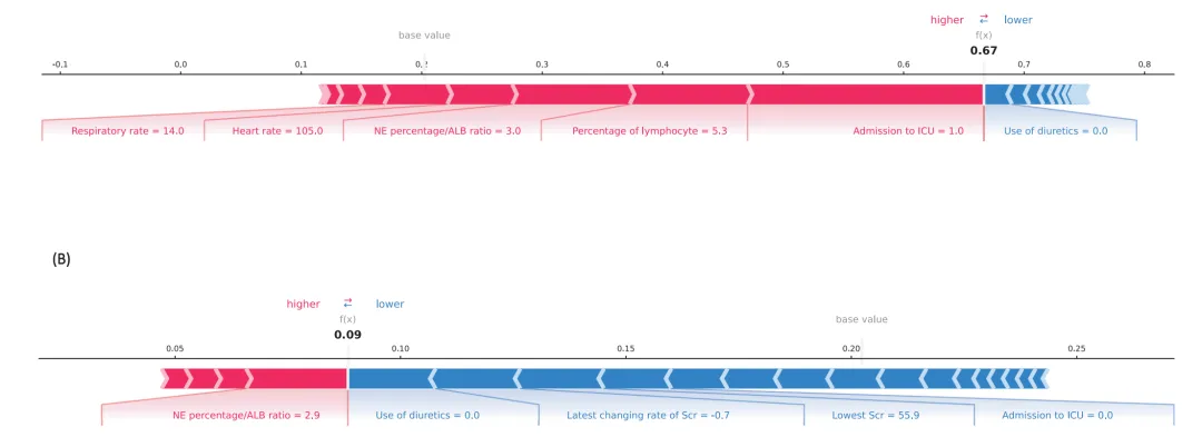
SHAP 的目标是:把任意复杂模型的预测结果,拆解成每个特征对该预测的贡献值。它输出的是一组“贡献分解”:
先有一个基线值(base value):可以理解为“在总体平均意义下的默认预测”。 每个特征都有一个 SHAP 值:表示该特征让预测相对基线“升高了多少”或“降低了多少”。 所有特征的 SHAP 值加起来 + 基线值 = 该样本最终预测(在模型输出空间里)。你可以把它理解成:机器学习模型的“个体列线图”——每个人都有一张只属于自己的贡献分解表,而不是一个全局固定的打分尺。 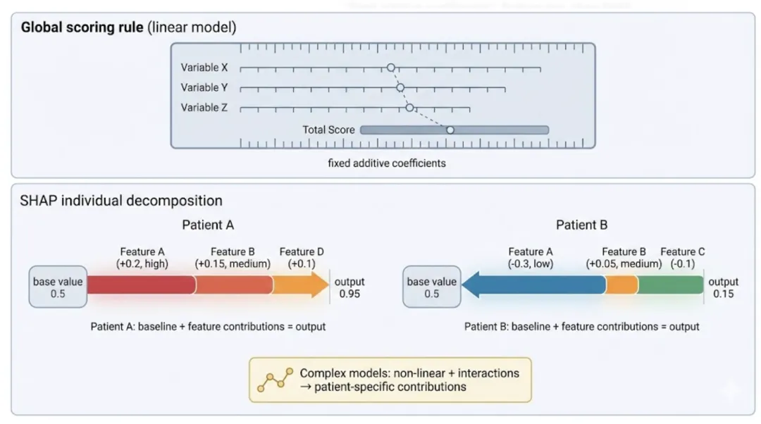
3. SHAP 可视化能回答临床最关心的三个问题
这个模型总体上“最重要”的变量是谁?用 SHAP summary plot(蜂群图) 或 bar plot(平均|SHAP|条形图)
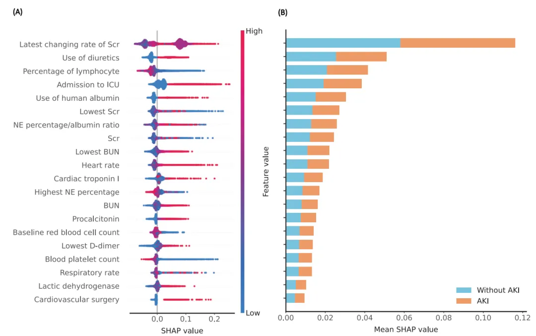
对某个具体病人,哪些因素把风险“推高/拉低”?用 waterfall plot(瀑布图) 或 force plot(力图)
某个变量到底是“怎么影响风险的”?是否非线性?是否存在阈值?用 dependence plot(依赖图)
❌错误说明:不能在机器学习模型的后面用列线图对模型进行使用,有不少已经发表的文章存在这类错误。机器学习模型要用SHAP等方法进行模型解释。误区:SHAP 值 ≠ 回归系数。系数是“整体平均线性效应”,SHAP 值是“在该模型、该样本上的边际贡献”。两者可以方向一致,但概念不同。误区:重要性高 ≠ 因果关系。SHAP 解释的是“模型如何使用变量做预测”,不是变量对结局的因果作用。尤其是回顾性数据、混杂和选择偏倚存在时,更要避免把“贡献”说成“导致”。

